Import and transform Relig-incom.csv
library(readxl)
library(tidyverse)
## -- Attaching packages --------------------------------------- tidyverse 1.3.1 --## v ggplot2 3.3.3 v purrr 0.3.4
## v tibble 3.1.1 v dplyr 1.0.6
## v tidyr 1.1.3 v stringr 1.4.0
## v readr 1.4.0 v forcats 0.5.1## -- Conflicts ------------------------------------------ tidyverse_conflicts() --
## x dplyr::filter() masks stats::filter()
## x dplyr::lag() masks stats::lag()rel_inc <- read_excel("relig-income.xlsx")
rel_inc <- read_excel(file.choose())
rel_inc_long <- rel_inc %>%
rename(religion = `Religious tradition`, n = `Sample Size`) %>%
pivot_longer(cols = -c(religion, n), # all but religion and n
names_to = "income",
values_to = "proportion") %>%
mutate(frequency = round(proportion * n))
rel_inc_long## # A tibble: 48 x 5
## religion n income proportion frequency
## <chr> <dbl> <chr> <dbl> <dbl>
## 1 Buddhist 233 Less than $30,000 0.36 84
## 2 Buddhist 233 $30,000-$49,999 0.18 42
## 3 Buddhist 233 $50,000-$99,999 0.32 75
## 4 Buddhist 233 $100,000 or more 0.13 30
## 5 Catholic 6137 Less than $30,000 0.36 2209
## 6 Catholic 6137 $30,000-$49,999 0.19 1166
## 7 Catholic 6137 $50,000-$99,999 0.26 1596
## 8 Catholic 6137 $100,000 or more 0.19 1166
## 9 Evangelical Protestant 7462 Less than $30,000 0.35 2612
## 10 Evangelical Protestant 7462 $30,000-$49,999 0.22 1642
## # ... with 38 more rowsVisualize using the Barplot
rel_inc_long <- rel_inc_long %>%
mutate(religion = case_when(
religion == "Evangelical Protestant" ~ "Ev. Protestant",
religion == "Historically Black Protestant" ~ "Hist. Black Protestant",
religion == 'Unaffiliated (religious "nones")' ~ "Unaffiliated",
TRUE ~ religion
))
rel_inc_long <- rel_inc_long %>%
mutate(religion = fct_rev(religion))
ggplot(rel_inc_long, aes(y = religion, x = frequency)) +
geom_col()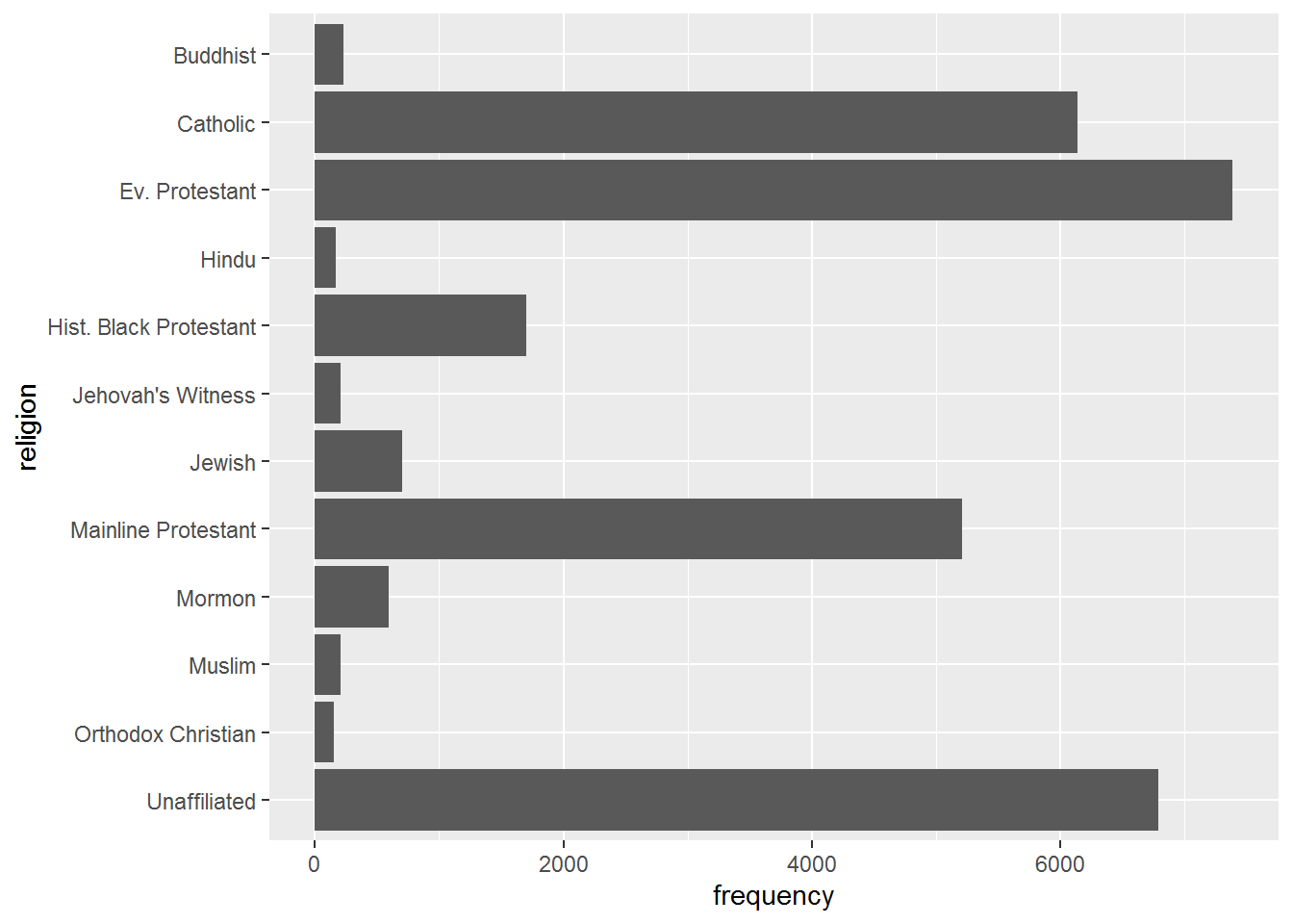 ## Fill Barplot with Income
ggplot(rel_inc_long, aes(y = religion, x = frequency, fill = income)) +
  geom_col()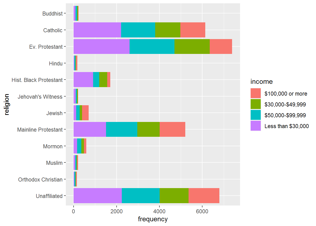
ggplot(rel_inc_long, aes(y = religion, x = frequency, fill = income)) +
geom_col(position = "fill") +
scale_fill_viridis_d()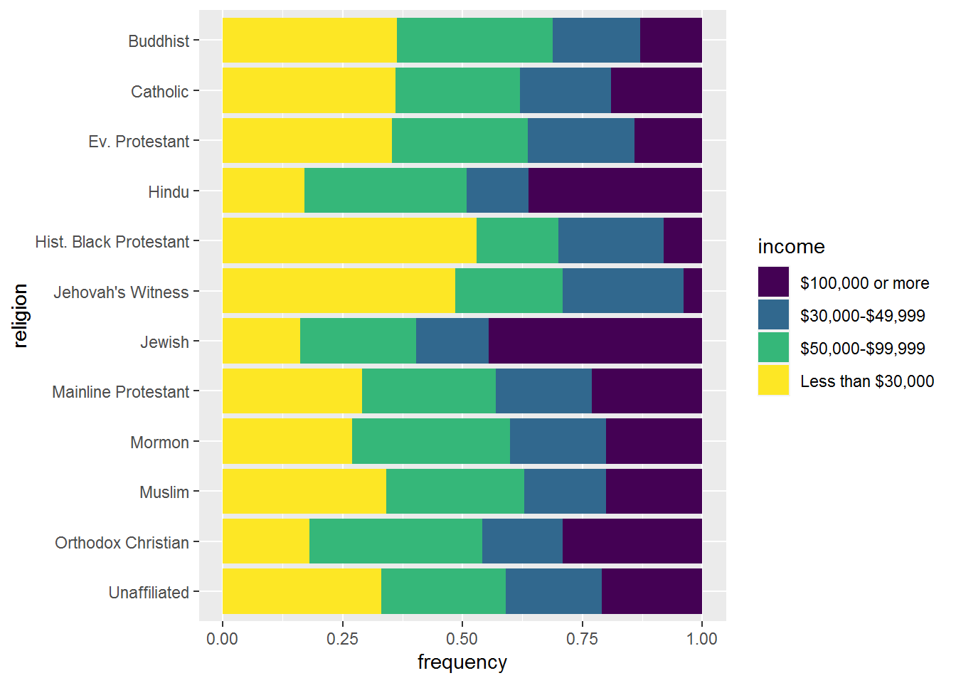 ## Change theme of the plot
ggplot(rel_inc_long, aes(y = religion, x = frequency, fill = income)) +
  geom_col(position = "fill") +
  scale_fill_viridis_d() +
  theme_minimal()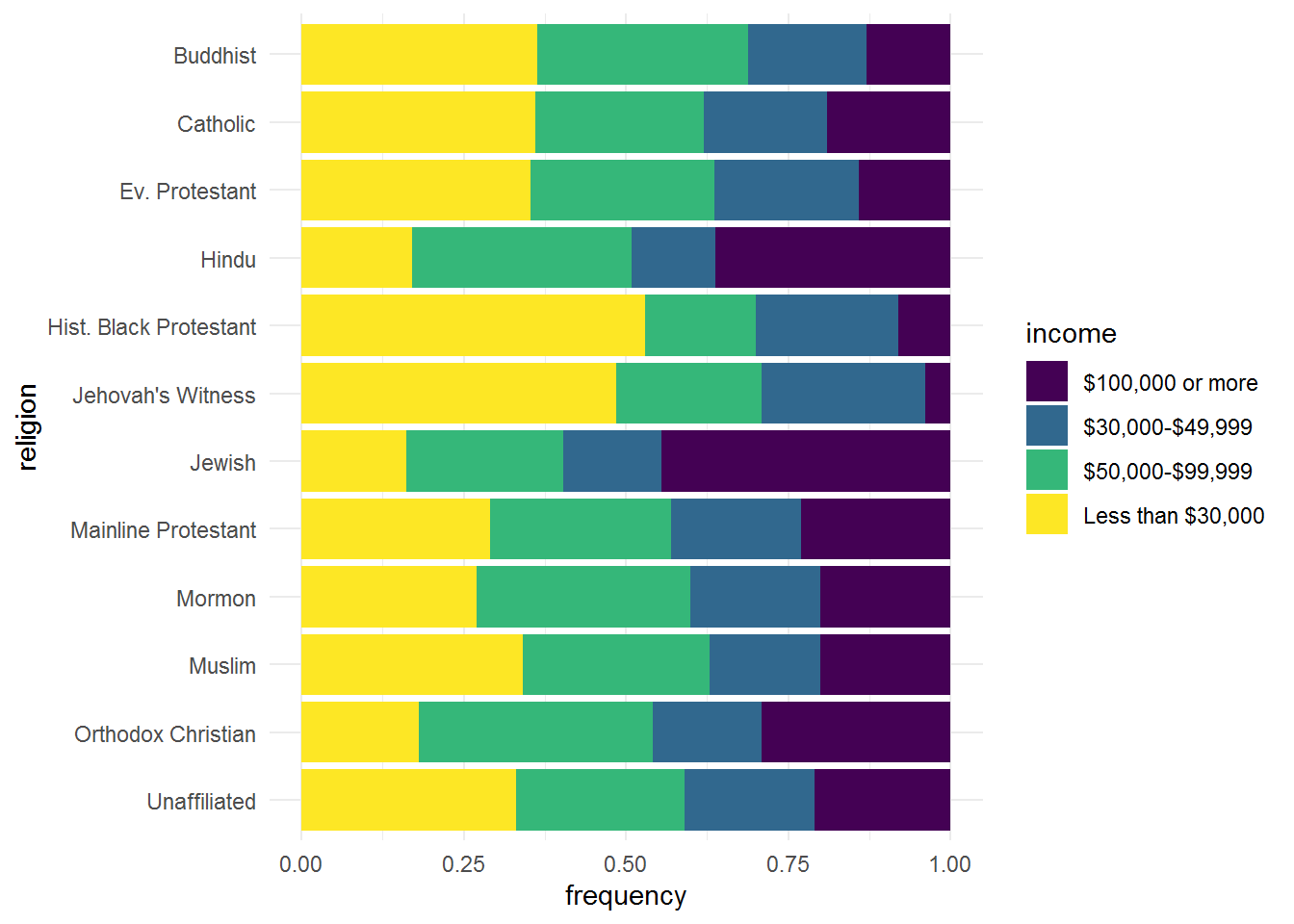
ggplot(rel_inc_long, aes(y = religion, x = frequency, fill = income)) +
  geom_col(position = "fill") +
  scale_fill_viridis_d() +
  theme_minimal() +
  theme(legend.position = "bottom")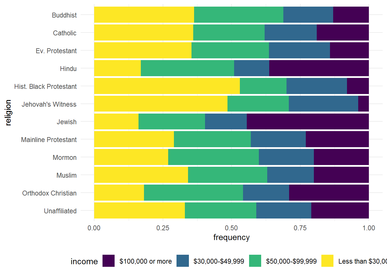
ggplot(rel_inc_long, aes(y = religion, x = frequency, fill = income)) +
  geom_col(position = "fill") +
  scale_fill_viridis_d() +
  theme_minimal() +
  theme(legend.position = "bottom") +
  guides(fill = guide_legend(nrow = 2, byrow = TRUE))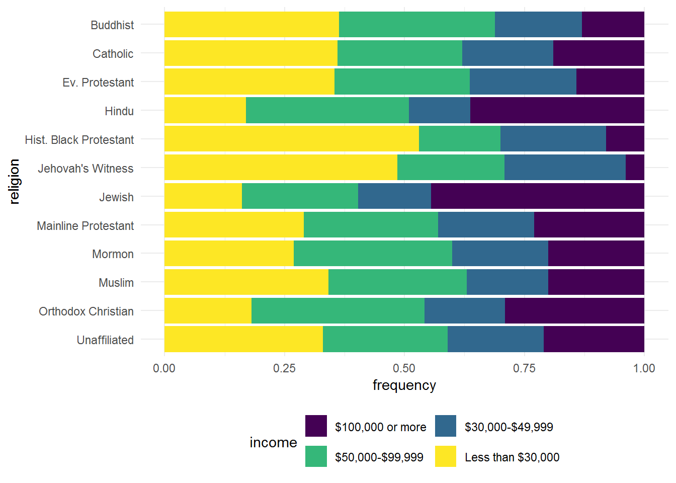
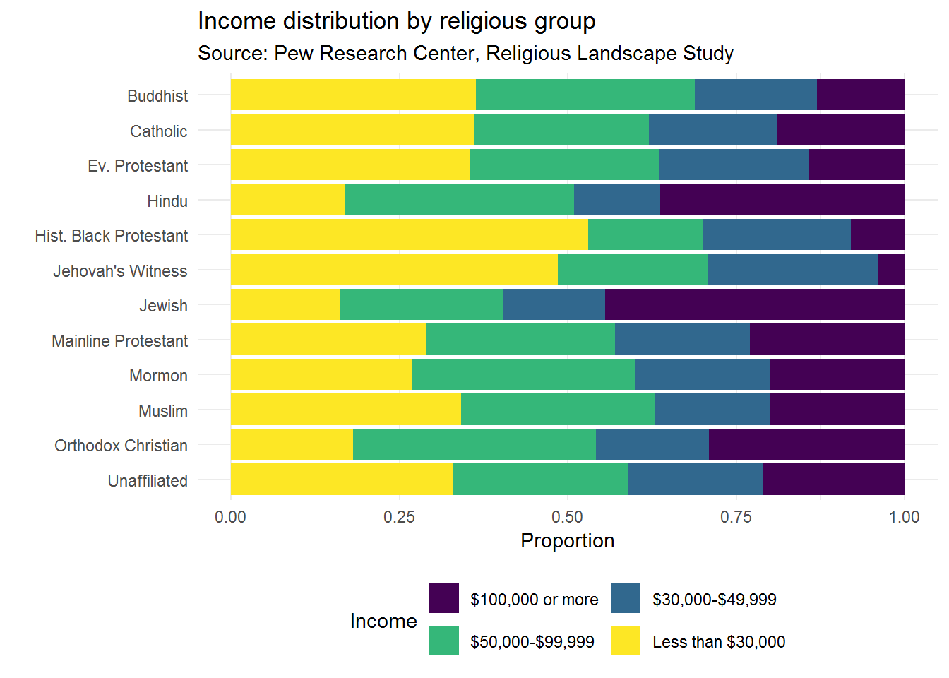
ggplot(rel_inc_long, aes(y = religion, x = frequency, fill = income)) +
  geom_col(position = "fill") +
  scale_fill_viridis_d() +
  theme_minimal() +
  theme(legend.position = "bottom") +
  guides(fill = guide_legend(nrow = 2, byrow = TRUE)) +
  labs(
    x = "Proportion", y = "",
    title = "Income distribution by religious group",
    subtitle = "Source: Pew Research Center, Religious Landscape Study",
    fill = "Income"
    )