Problem definition

A professor of machine learning is planning to get married to his long-time girlfriend. He has never shopped for diamonds before. In the mall, he was confronted with a dizzying array of diamond characteristics, configurations, and pricing. His quick search revealed that diamonds are primarily characterized by 4C viz. Color, Cut, Carat Weight and Clarity besides Polish, Symmetry, and certification. He scrapped the web to collect information from three different wholesaler websites to build his pricing model to ensure he does not get cheated while purchasing the diamond ring. Build a Linear Regression Model to predict the price of the diamond ring of his interest.

Import data

## Rows: 440
## Columns: 9
## $ Carat         <dbl> 92, 92, 82, 81, 9, 87, 8, 84, 8, 8, 85, 83, 82, 82, 8, 9~
## $ Colour        <chr> "I", "I", "F", "G", "J", "F", "D", "F", "D", "D", "G", "~
## $ Clarity       <chr> "SI2", "SI2", "SI2", "SI1", "VS2", "SI2", "SI2", "SI1", ~
## $ Cut           <chr> "G", "V", "I", "I", "V", "I", "I", "G", "V", "V", "I", "~
## $ Certification <chr> "AGS", "AGS", "GIA", "GIA", "GIA", "AGS", "GIA", "GIA", ~
## $ Polish        <chr> "V", "G", "X", "X", "V", "G", "V", "V", "V", "V", "V", "~
## $ Symmetry      <chr> "V", "G", "X", "V", "V", "V", "V", "V", "V", "X", "V", "~
## $ Price         <dbl> 3000, 3000, 3004, 3004, 3006, 3007, 3008, 3010, 3012, 30~
## $ Wholesaler    <dbl> 1, 1, 1, 1, 1, 1, 1, 1, 1, 1, 1, 1, 1, 1, 1, 1, 1, 1, 1,~

We use exploratory graphs in data analysis to understand data properties, find patterns in data, suggest modeling strategies.

Univariate Analysis of Metric Data

Univariate EDA for a quantitative variable is a way to make preliminary assessments about the population distribution of the variable using the data of the observed sample.

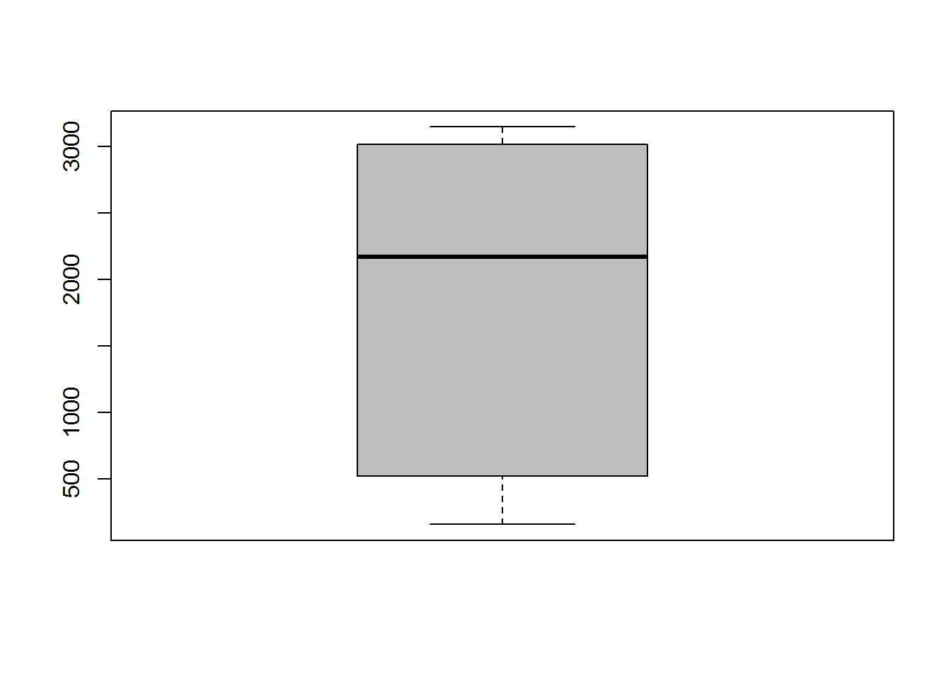
Price

The distribution of price shows two different range. First range is between $100-$700 and the second one is between almost $1800-$3300. With this information, we are not able to found that why there are no price data in range $800-$1700. Median of price is $2169 and the mean is $1717. The professor’s diamond ring price is $3100 which almost near the maximum price of the price data set. It means that either the diamond ring is precious enough or the professor will get cheated. We should analyze other specification of diamond to found whether they are at the precious level or not.

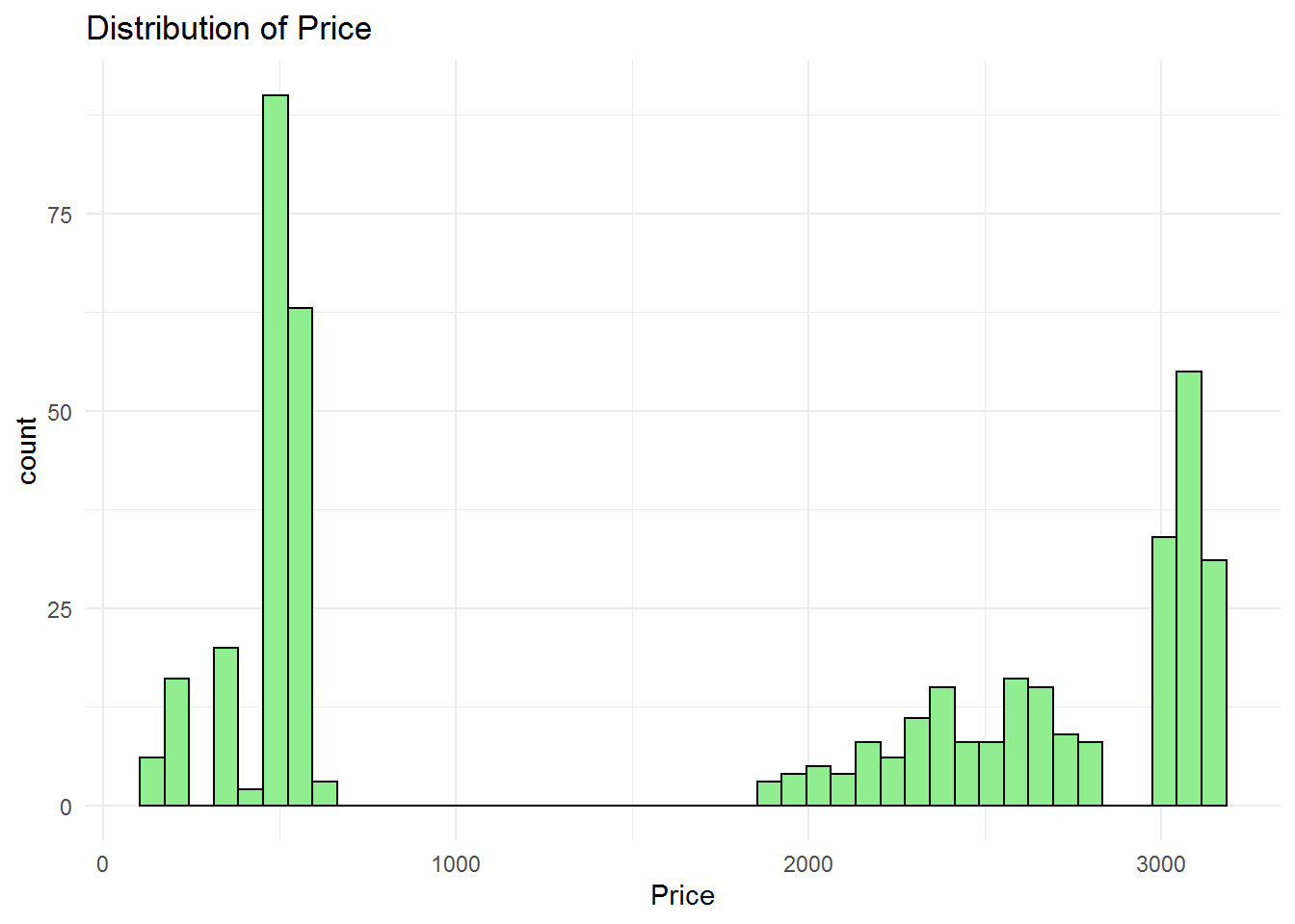
##    Min. 1st Qu.  Median    Mean 3rd Qu.    Max. 
##     160     520    2169    1717    3012    3145

Carat

Let’s look at the another parameter of diamond ring, Carat.

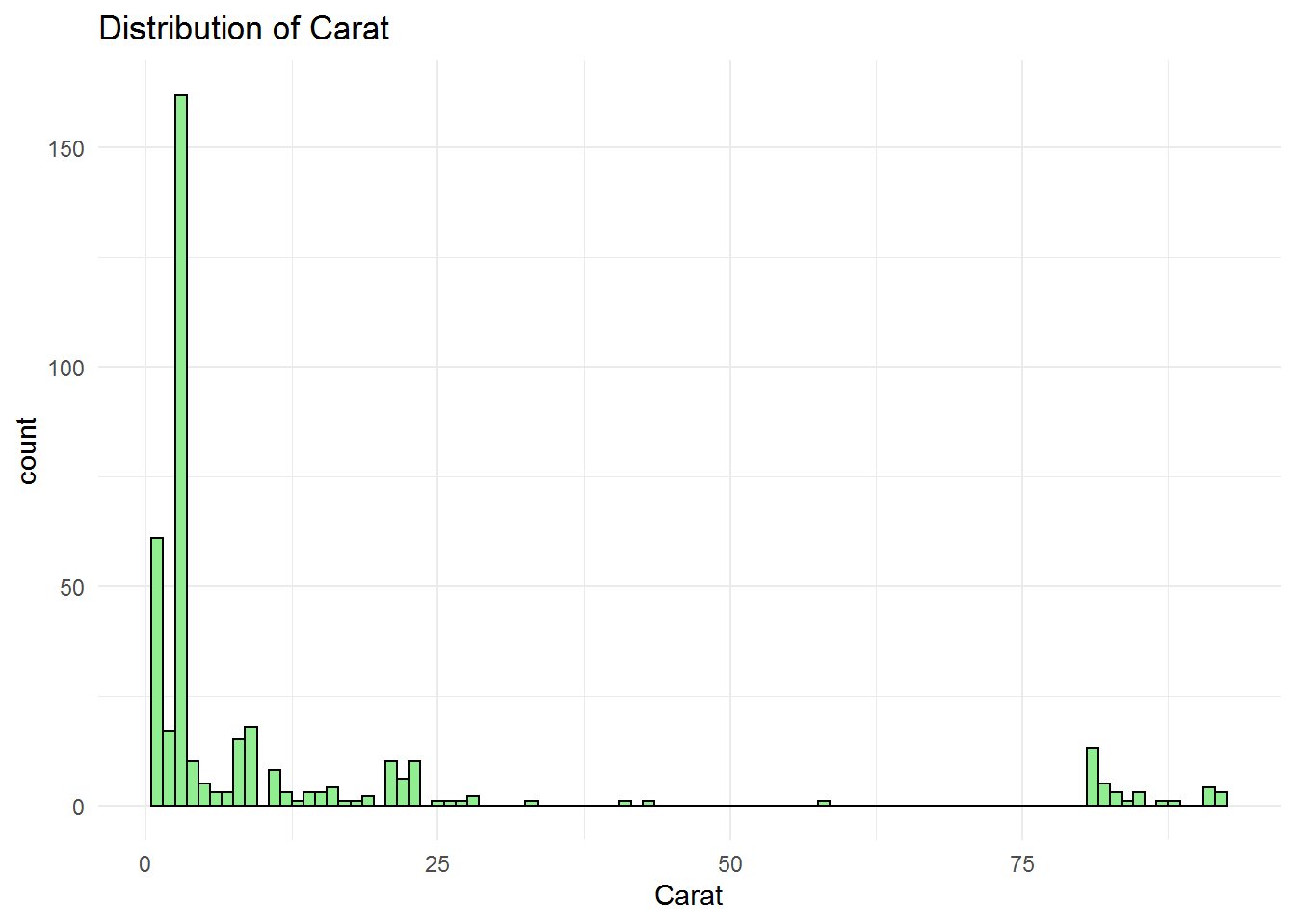
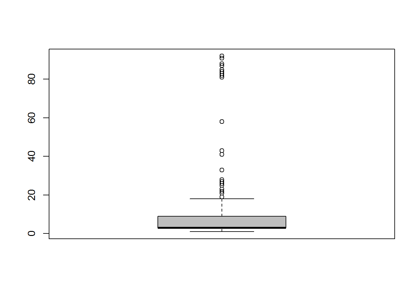
##    Min. 1st Qu.  Median    Mean 3rd Qu.    Max.    NA's 
##    1.00    3.00    3.00   13.05    9.00   92.00      51

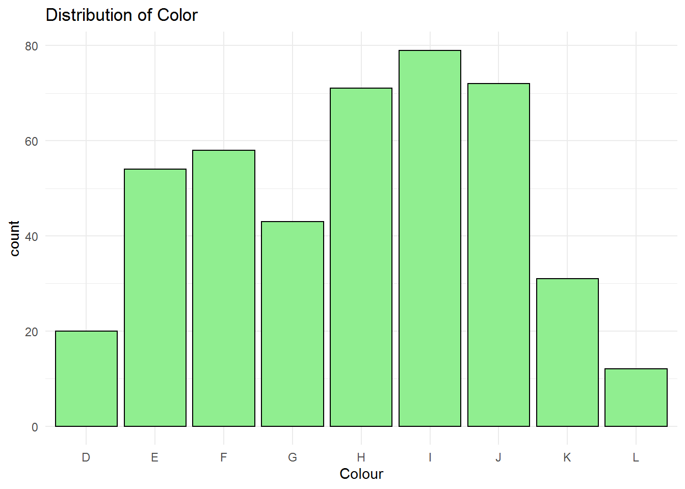
Colour

Acording to the data, Colour includes D, E, F, G, H, I, G, K, and L. D-F: Colorless G-I: Near Colorless J-K: Faint Yellow L-N: Very light yellow O-S: Light Yellow T-Z: Yellow

The mode is for I and the least frequency relates to colour L. The professor wants to buy a diamond ring with colour J , Faint Yellow, which is the second most popular ring among all. However, with this univariate analysis we cannot found the relation between the most frequent colours and the price to help the professor. we need a bivariat analysis to figure out the estimation of the price based on the colour Faint Yellow.

##    Length     Class      Mode 
##       440 character character

Clarity

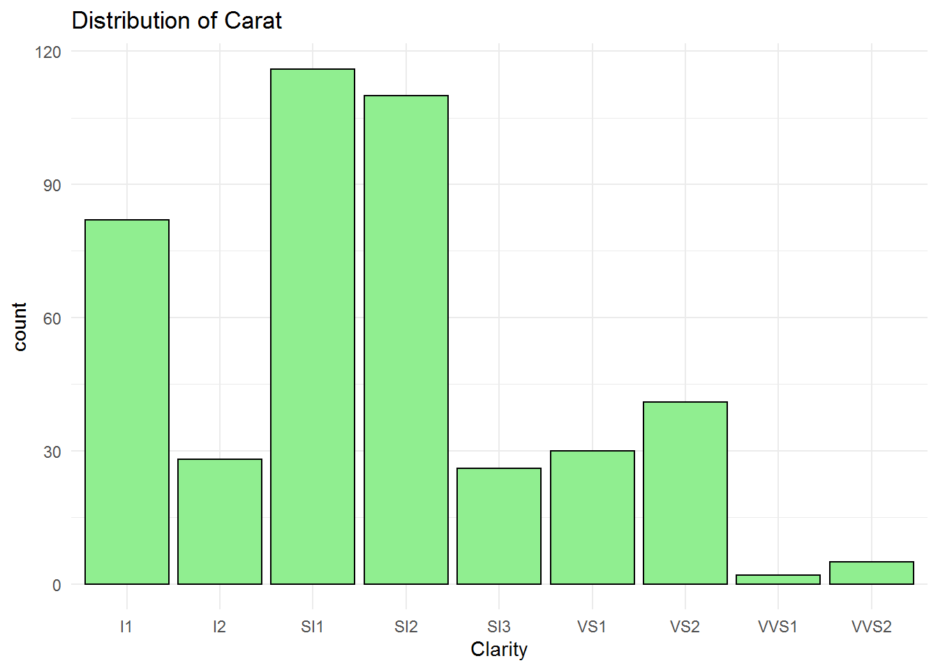
I1: very few inclusions visible to naked eye I2: few inclusions visible to naked eye SI1: very very few inclusions at 10X SI2: very few inclusions at 10X SI3: several inclusions at 10X VS1: few inclusions at 30X VS: several inclusions at 30X VVS1: very very few inclusions at 30X VVS2: very few inclusions at 30X

Figure shows that the most frequent clarity is SI1 which is very very few inclusions at 10X. The professor wants to buy a ring with SI2 that has very few inclusions at 10X and is the second most frequent type of ring among all. Again, we need a bivariate analysis to see the distribution of the dimaond ring price based on different clarity features.

##    Length     Class      Mode 
##       440 character character

Cut

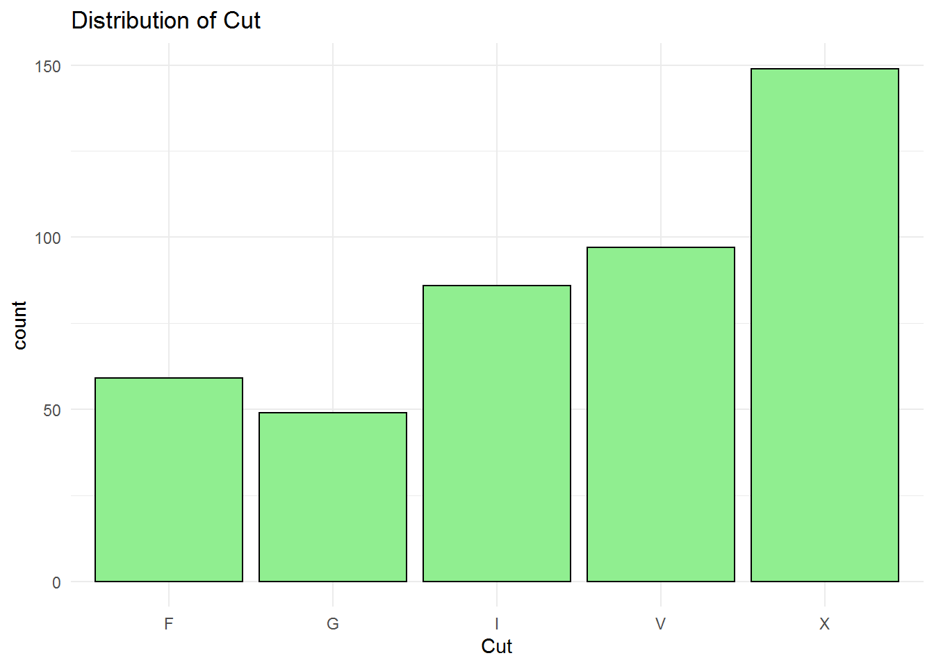
F: Fair G: Good I: Ideal V: Very Good X: Excellent

Type x of cut is the most frequent among others which represent the excellent cut. The professor is going to buy a very good cut which is the second most frequent cut type.

##    Length     Class      Mode 
##       440 character character

Certification

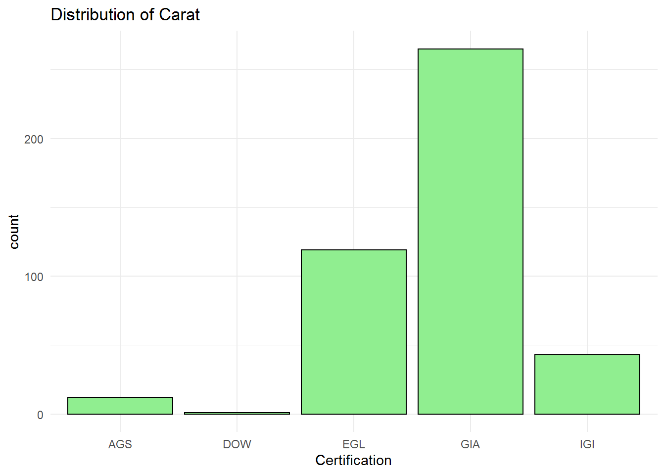
The mode of certification data is GIA and also the professor wants to buy a diamond ring with GIA certification. Like previous analysis, univariate investigation cannot help us to find the relationship between the price and type of certification.

##    Length     Class      Mode 
##       440 character character

Polish

F: Fair G: Good I: Ideal V: Very Good X: Excellent

Polish classification is similar to the cut code. As can be seen in the bar chart, very good and good are the most nd second most ones. The professor ring has good polish that seems to be a good choice.

##    Length     Class      Mode 
##       440 character character

Symmetry

F: Fair G: Good I: Ideal V: Very Good X: Excellent

Symmetry classification is also similar to the cut code and polish. Very good and good symmetry are popular. The professor choice is very good which the mode of the symmetry variable.

##    Length     Class      Mode 
##       440 character character

Price vs Carat

The correlation between the price and the Carat is shown in the following figure and the linear regression model and coefficents are also calculated. For the professor choice that Carat is 0.9, the price $3100 seeems fair according to these analysis. The p-values are also significant that makes we sure that the linear regression model is reliable.

## `geom_smooth()` using formula 'y ~ x'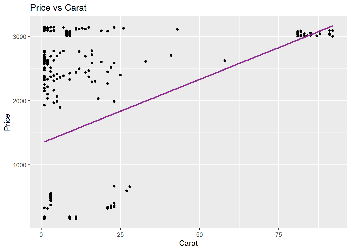

## # A tibble: 2 x 5
##   term        estimate std.error statistic  p.value
##   <chr>          <dbl>     <dbl>     <dbl>    <dbl>
## 1 (Intercept)   1340.      64.1      20.9  1.48e-65
## 2 Carat           19.8      2.40      8.25 2.56e-15

\[\widehat{Price}_{i} = 1339.88 + 19.82 \times Carat_{i}\]

Price vs Colour

The correlation between the price and the Colour is shown in the following figure and the linear regression model and coefficents are also calculated. For the professor choice that Colour is J, we can see a range of price implyng that there is a need to more analysis on other variables using the multiple regression. The p-values for some colours are not significant significant showing that this model is not significant enough in overall.

## `geom_smooth()` using formula 'y ~ x'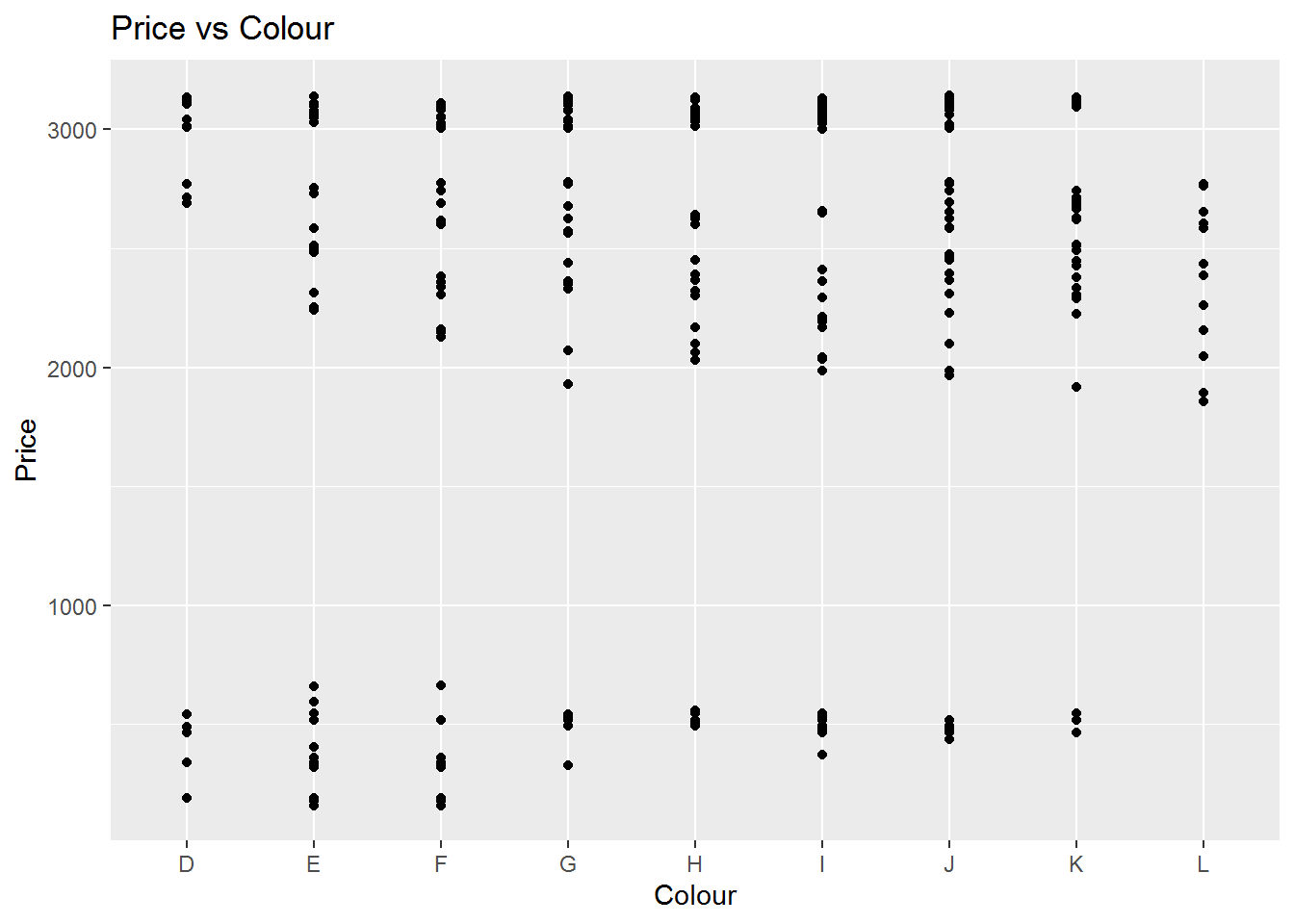

## # A tibble: 9 x 5
##   term        estimate std.error statistic  p.value
##   <chr>          <dbl>     <dbl>     <dbl>    <dbl>
## 1 (Intercept)   2316.       254.     9.13  2.74e-18
## 2 ColourE       -764.       297.    -2.57  1.04e- 2
## 3 ColourF       -982.       294.    -3.34  9.17e- 4
## 4 ColourG       -148.       307.    -0.481 6.31e- 1
## 5 ColourH       -874.       287.    -3.04  2.50e- 3
## 6 ColourI       -766.       284.    -2.70  7.30e- 3
## 7 ColourJ       -535.       287.    -1.87  6.27e- 2
## 8 ColourK         42.1      326.     0.129 8.97e- 1
## 9 ColourL         52.3      414.     0.126 9.00e- 1

Price vs Clarity

The analysis of price vs clarity also seems like the Colour one results. For instance, for the clarity of S12 which is the professor diamond ring choice, we can see a wide range of actual prices. This means that there are other variables affecting the price.

## `geom_smooth()` using formula 'y ~ x'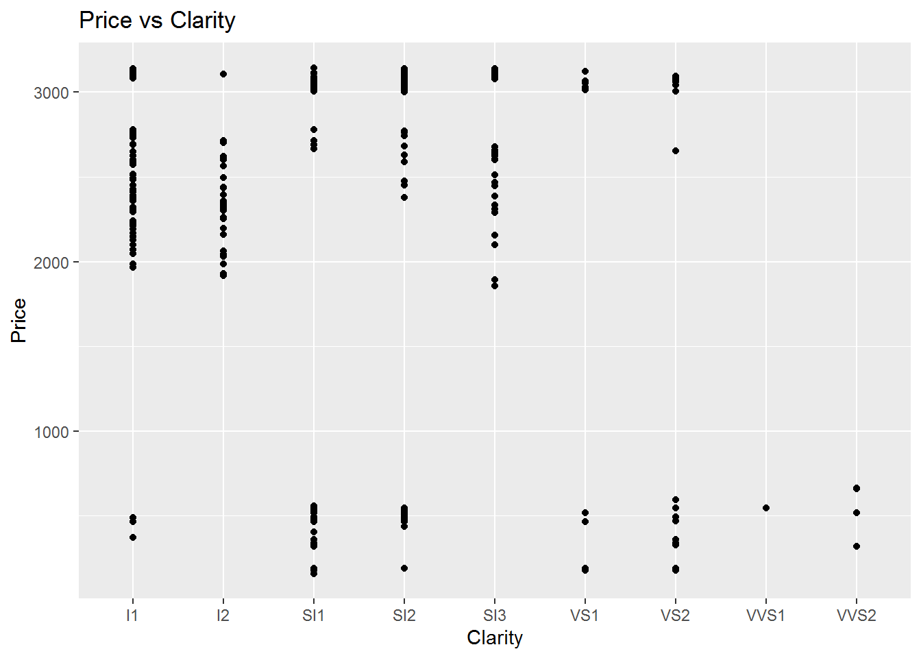

## # A tibble: 9 x 5
##   term        estimate std.error statistic  p.value
##   <chr>          <dbl>     <dbl>     <dbl>    <dbl>
## 1 (Intercept)   2543.       108.    23.6   1.82e-79
## 2 ClarityI2     -201.       214.    -0.940 3.48e- 1
## 3 ClaritySI1   -1496.       141.   -10.6   1.69e-23
## 4 ClaritySI2    -569.       143.    -3.99  7.79e- 5
## 5 ClaritySI3      76.2      220.     0.347 7.29e- 1
## 6 ClarityVS1   -1405.       209.    -6.74  5.17e-11
## 7 ClarityVS2   -1655.       187.    -8.85  2.27e-17
## 8 ClarityVVS1  -1996.       700.    -2.85  4.54e- 3
## 9 ClarityVVS2  -1979.       450.    -4.39  1.40e- 5

Price vs Cut

The correlation between the price and the Cut is shown in the following figure and the linear regression model and coefficents are also calculated. We can see that coefficents of linear regression are significant although the plot shows the gap between the prices of each cut category. Therefore, we need more analysis.

## `geom_smooth()` using formula 'y ~ x'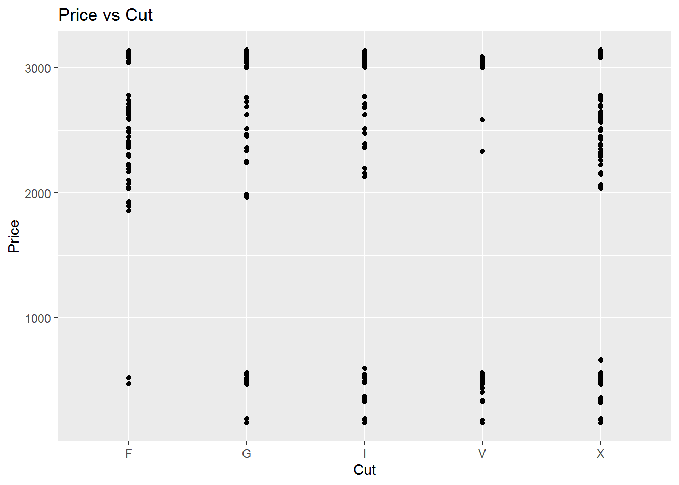

## # A tibble: 5 x 5
##   term        estimate std.error statistic  p.value
##   <chr>          <dbl>     <dbl>     <dbl>    <dbl>
## 1 (Intercept)    2455.      145.     16.9  1.07e-49
## 2 CutG           -409.      215.     -1.90 5.82e- 2
## 3 CutI           -723.      188.     -3.84 1.42e- 4
## 4 CutV          -1277.      184.     -6.94 1.44e-11
## 5 CutX           -797.      171.     -4.65 4.43e- 6

Price vs Certification

The correlation between the price and the Certification is shown in the following figure and the linear regression model and coefficents are also calculated. For the professor choice which is GIA cetification, the coefficient of regression is reliable but the plot shows a wide range of price meaning tat other variables effect should be considered.

## `geom_smooth()` using formula 'y ~ x'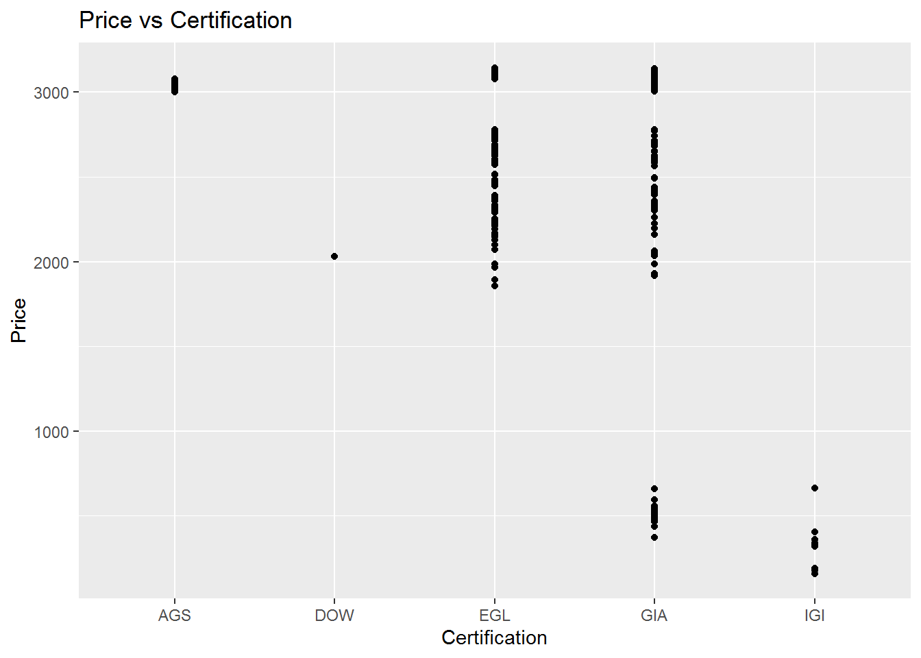

## # A tibble: 5 x 5
##   term             estimate std.error statistic  p.value
##   <chr>               <dbl>     <dbl>     <dbl>    <dbl>
## 1 (Intercept)         3033.      265.     11.4  1.28e-26
## 2 CertificationDOW   -1002.      957.     -1.05 2.96e- 1
## 3 CertificationEGL    -356.      279.     -1.28 2.02e- 1
## 4 CertificationGIA   -1574.      271.     -5.80 1.30e- 8
## 5 CertificationIGI   -2768.      300.     -9.22 1.31e-18

Price vs Polish

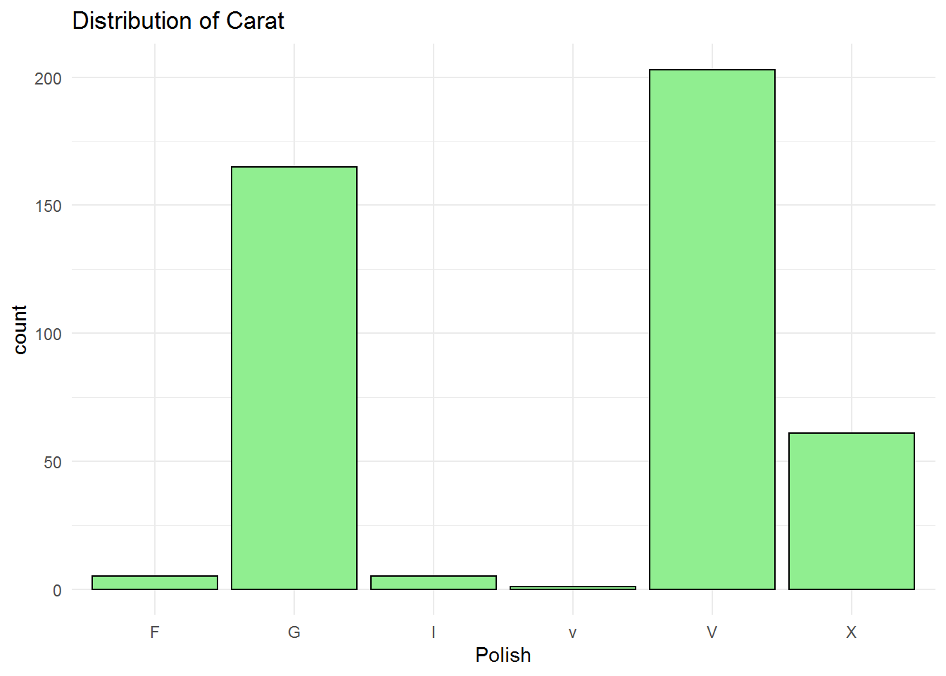
The correlation between the price and the Polish is shown in the following figure and the linear regression model and coefficents are also calculated. Most of the regression coefficients are insignificant. Moreover, for the professor choice, Good Polish, the coefficient is not significant.

## `geom_smooth()` using formula 'y ~ x'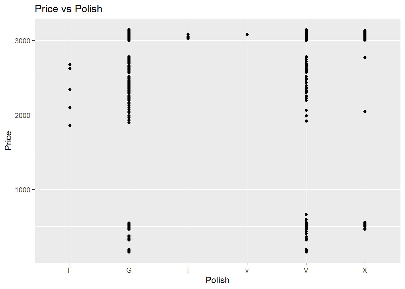

## # A tibble: 6 x 5
##   term        estimate std.error statistic    p.value
##   <chr>          <dbl>     <dbl>     <dbl>      <dbl>
## 1 (Intercept)    2319.      516.     4.49  0.00000907
## 2 PolishG        -404.      524.    -0.771 0.441     
## 3 PolishI         729.      730.     0.998 0.319     
## 4 Polishv         762.     1264.     0.603 0.547     
## 5 PolishV        -715.      523.    -1.37  0.172     
## 6 PolishX        -940.      537.    -1.75  0.0808

Price vs Symmetry

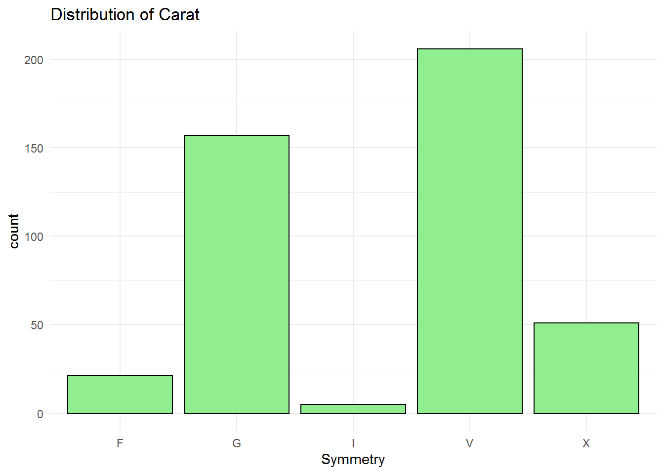
The correlation between the price and the Polish is shown in the following figure and the linear regression model and coefficents are also calculated. Most of the regression coefficients are insignificant but the Symmetry V, which is the professor’s diamond ring specification, we can see a significant coefficient. However, the plot shows a wide range of price meaning that effect of other variables should be considered.

## `geom_smooth()` using formula 'y ~ x'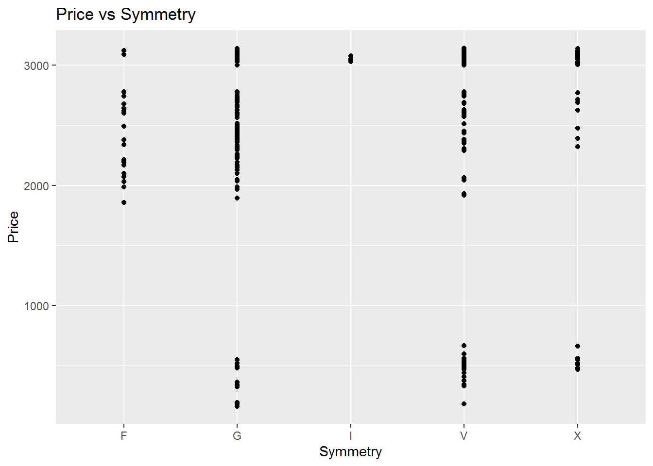

## # A tibble: 5 x 5
##   term        estimate std.error statistic  p.value
##   <chr>          <dbl>     <dbl>     <dbl>    <dbl>
## 1 (Intercept)    2432.      250.      9.74 2.00e-20
## 2 SymmetryG      -538.      266.     -2.02 4.36e- 2
## 3 SymmetryI       615.      569.      1.08 2.80e- 1
## 4 SymmetryV      -967.      262.     -3.69 2.53e- 4
## 5 SymmetryX      -673.      297.     -2.27 2.38e- 2

## # A tibble: 35 x 5
##    term        estimate std.error statistic  p.value
##    <chr>          <dbl>     <dbl>     <dbl>    <dbl>
##  1 (Intercept)   1902.     663.      2.87   4.39e- 3
##  2 Carat           22.8      1.81   12.6    3.33e-30
##  3 ColourE       -237.     204.     -1.16   2.47e- 1
##  4 ColourF       -281.     203.     -1.38   1.68e- 1
##  5 ColourG         10.9    206.      0.0530 9.58e- 1
##  6 ColourH       -417.     202.     -2.06   3.99e- 2
##  7 ColourI       -381.     203.     -1.88   6.13e- 2
##  8 ColourJ       -295.     209.     -1.41   1.59e- 1
##  9 ColourK        114.     239.      0.477  6.34e- 1
## 10 ColourL       -227.     304.     -0.747  4.55e- 1
## # ... with 25 more rows